Closed Form Precision
Previous: Measuring Precision
Symmetric Bivariate Normal = Rayleigh Distribution
After factoring out the known sources of asymmetry in the bivariate normal model we believe that shot groups are sufficiently symmetric that we can assume \(\sigma_x = \sigma_y\). In this case the dispersion of shots is modeled by a symmetric bivariate normal, which is equivalent[1] to the Rayleigh distribution, described by a single parameter σ.
NB: It is common to describe normal distributions using variance, or \(\sigma^2\), because variances have some convenient linear characteristics that are lost when we take the square root. For similar reasons many prefer to describe the Rayleigh distribution using a parameter \(\gamma = \sigma^2\). To clarify our parameterization the σ we will be describing is the standard deviation of the bivariate normal distribution, and the parameter that produces the following pdf for the Rayleigh distribution:
- \(\frac{x}{\sigma^2}e^{-x^2/2\sigma^2}\)
Where the bivariate normal distribution describes the coordinates (x, y) of shots on target, the Rayleigh distribution describes the distance, or radius, \(r_i = \sqrt{(x_i - \bar{x})^2 + (y_i - \bar{y})^2}\) of those shots from the center point of impact.
Estimating σ
The Rayleigh distribution provides closed form expressions for precision. However, when estimating σ from sample sets we will most often use methods associated with the normal distribution for one essential reason: We never observe the true center of the distribution. When we calculate the center of a group on a target it will almost certainly be some distance from the true center, and thus underestimate the true distance of the sample shots to the distribution center. (Average distance from sample center to true center is listed in the second column of Media:Sigma1ShotStatistics.ods.) The Rayleigh model describes the distribution of shots from the (unobservable) true center. When the center is unknown we have to use the sample center, and we fall back on characteristics of the normal distribution with unknown mean.
Correction Factors
The following three correction factors will be used throughout this statistical inference and deduction.
Note that all of these correction factors are > 1, are significant for very small n, and converge towards 1 as \(n \to \infty\). Their values are listed for n up to 100 in Media:Sigma1ShotStatistics.ods. File:SymmetricBivariate.c uses Monte Carlo simulation to confirm that their application produces valid corrected estimates.
Bessel correction factor
The Bessel correction removes bias in sample variance.
- \(c_{B}(n) = \frac{n}{n-1}\)
Gaussian correction factor
The Gaussian correction (sometimes called \(c_4\)) removes bias introduced by taking the square root of variance.
- \(\frac{1}{c_{G}(n)} = \sqrt{\frac{2}{n-1}}\,\frac{\Gamma\left(\frac{n}{2}\right)}{\Gamma\left(\frac{n-1}{2}\right)} \, = \, 1 - \frac{1}{4n} - \frac{7}{32n^2} - \frac{19}{128n^3} + O(n^{-4})\)
The third-order approximation is adequate. The following spreadsheet formula gives a more direct calculation: \(c_{G}(n)\) =EXP(LN(SQRT(2/(N-1))) + GAMMALN(N/2) - GAMMALN((N-1)/2))
Rayleigh correction factor
The unbiased estimator for the Rayleigh distribution is also for \(\sigma^2\). The following corrects for the concavity introduced by taking the square root to get σ.
- \(c_{R}(n) = 4^n \sqrt{\frac{n}{\pi}} \frac{ N!(N-1)!} {(2N)!}\) [2]
To avoid overflows this is better calculated using log-gammas, as in the following spreadsheet formula: =EXP(LN(SQRT(N/PI())) + N*LN(4) + GAMMALN(N+1) + GAMMALN(N) - GAMMALN(2N+1))
Data
In the following formulas assume that we are looking at a target reflecting n shots and that we are able to determine the center coordinates x and y for each shot.
(One easy way to compile these data is to process an image of the target through a program like OnTarget Precision Calculator.)
Variance Estimates
For a single axis the unbiased estimate of variance for a normal distribution is \(s_x^2 = \frac{\sum (x_i - \bar{x})^2}{n-1} \), from which the unbiased estimate of standard deviation is \(\widehat{\sigma_x} = c_G(n) \sqrt{(s_x^2)}\).
Since we are assuming that the shot dispersion is jointly independent and identically distributed along the x and y axes we improve our estimate by aggregating the data from both dimensions. I.e., we look at the average sample variance \(s^2 = (s_x^2 + s_y^2)/2\), and \(\hat{\sigma} = c_G(2n-1) \sqrt{s^2}\). This turns out to be identical to the Rayleigh estimator.
Rayleigh Estimates
The Rayleigh distribution describes the random variable R defined as the distance of each shot from the center of the distribution. Again, we never get to observe the true center, so we begin by calculating the sample center \((\bar{x}, \bar{y})\). Then for each shot we can compute the sample radius \(r_i = \sqrt{(x_i - \bar{x})^2 + (y_i - \bar{y})^2}\).
The unbiased Rayleigh estimator is \(\widehat{\sigma_R^2} = c_B(n) \frac{\sum r_i^2}{2n} = \frac{c_B(n)}{2} \overline{r^2}\), which is literally a restatement of the combined variance estimate \(s^2\). Hence the unbiased parameter estimate is once again \(\hat{\sigma} = c_G(2n-1) \sqrt{\widehat{\sigma^2}}\)
Confidence Intervals
Siddiqui[3] shows that the confidence intervals are given by the \(\chi^2\) distribution with 2n degrees of freedom. However this assumes we know the true center of the distribution. We lose two degrees of freedom (one in each dimension) by using the sample center, so we actually have only 2(n - 1) degrees of freedom. (Here again we will get the same equations if we instead follow the derivation of confidence intervals for the combined variance \(s^2\).)
To find the (1 - α) confidence interval, first find \(\chi_1^2, \ \chi_2^2\) where:
- \(Pr(\chi^2(2(n-1)) \leq \chi_1^2) = \alpha/2, \quad Pr(\chi^2(2(n-1)) \leq \chi_2^2) = 1 - \alpha/2\)
For example, using spreadsheet functions we have \(\chi_1^2\) = CHIINV(α/2, 2n-2),\(\quad \chi_2^2\) = CHIINV((1-α/2), 2n-2).
Now the confidence intervals are given by the following:
- \(s^2 \in \left[ \frac{2(n-1) s^2}{\chi_2^2}, \ \frac{2(n-1) s^2}{\chi_1^2} \right]\), or in equivalent Rayleigh terms \(\widehat{\sigma_R^2} \in \left[ \frac{\sum r^2}{\chi_2^2}, \ \frac{\sum r^2}{\chi_1^2} \right]\)
Using the more convenient Rayleigh expression the confidence interval for the precision parameter is:
- \(\widehat{\sigma} \in \left[ c_G(2n-1) \sqrt{\frac{\sum r^2}{\chi_2^2}}, \ c_G(2n-1) \sqrt{\frac{\sum r^2}{\chi_1^2}} \right]\)
How large a sample do we need?
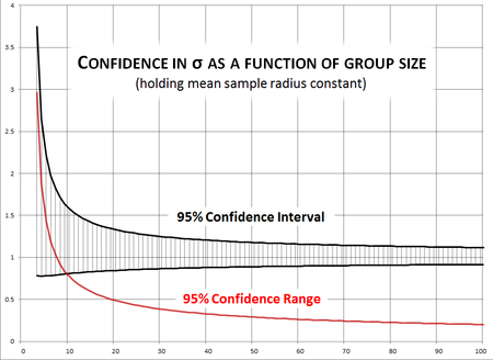
Note that confidence intervals are a function of both the sample size and the average radius in the sample. If we hold the mean sample radius constant we can see how the confidence interval tightens with sample size. The adjacent chart shows the 95% confidence intervals for σ when the estimate is 1.0 and the mean sample radius is held constant at \(\overline{r^2} = 2\).
With a sample of 10 shots our confidence interval is 77% as large as the parameter σ itself. At 20 it's just under 50%. It takes a group of 66 shots to get it under 25% and 100 to get it to 20% of the estimated σ.
Using σ
The σ we have carefully sampled and estimated is the parameter for the Rayleigh distribution with probability density function \(\frac{x}{\sigma^2}e^{-x^2/2\sigma^2}\). The associated Cumulative Distribution Function gives us the probability that a shot falls within a given radius of the center:
- \(Pr(r \leq \alpha) = 1 - e^{-\alpha^2 / 2 \sigma}\)
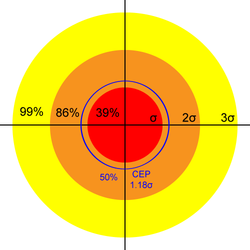
Therefore, we expect 39% of shots to fall within a circle of radius σ, 86% within 2σ, and 99% within 3σ.
Using the characteristics of the Rayleigh distribution we can immediately compute the three most useful precision measures:
Mean Radius (MR)
Mean Radius \(MR = \sigma \sqrt{\frac{\pi}{2}} \ \approx 1.25 \ \sigma\).
\(1 - e^{-\frac{\pi}{4}} \approx 54\%\) of shots should fall within the mean radius. 96% of shots should fall within the Mean Diameter (MD = 2 MR).
The expected sample MR of a group of size n is
- \(MR_n = \sigma \sqrt{\frac{\pi}{2 c_{B}(n)}}\ = \sigma \sqrt{\frac{\pi (n - 1)}{2 n}}\)
(This sample size adjustment doesn't use the Gaussian correction factor because the mean radius is not an estimator for σ, even though in the limit the true value of one is a constant product of the other.)
Circular Error Probable (CEP)
Circular Error Probable \(CEP = \sigma \sqrt{\ln(4)} \ \approx 1.18 \ \sigma\). 50% of shots should fall within the circular error probable.
In theory CEP is the median radius, but especially for small n the sample median is a very bad estimator for true median. Nevertheless, if you want to know the expected sample median radius of a group of size n it turns out the following is a good estimate:
- \(CEP_n = \sigma \frac{\sqrt{\ln(4)}}{c_{G}(n) c_{R}(n)}\)
Summary Probabilities
| Name | Multiple of σ | Shots Covered |
|---|---|---|
| 1 | 39% | |
| CEP | 1.18 | 50% |
| MR | 1.25 | 54% |
| 2 | 86% | |
| MD | 2.5 | 96% |
| 3 | 99% |
Typical values of σ
A lower bound on σ is probably that displayed by rail guns in 100-yard competition. On average they can place 10 rounds into a quarter-inch group, which as we will see shortly suggests σ = 0.070MOA, or under 0.025mil.
The U.S. Precision Sniper Rifle specification requires a statistically significant number of 10-round groups fall under 1MOA. This means σ = 0.28MOA, or under 0.1mil.
The specification for the M110 semi-automatic sniper rifle (MIL-PRF-32316) as well as the M24 sniper rifle (MIL-R-71126) requires MR below 0.65SMOA, which means σ = 0.5MOA. The latter spec indicates that an M24 barrel is not considered worn out until MR exceeds 1.2MOA, or σ = 1MOA!
XM193 ammunition specifications require 10-round groups to fall under 2MOA. This means σ = 0.6MOA or 0.2mil, and it is a good minimum precision standard for light rifles.
References
Next: Examples

